
Metaheuristic Identification for an Analytic Dynamic Model of a Delta Robot with Experimental Verification

1
Department of Mechanical Engineering, Chung-Ang University, 84 Heukseok-ro, Dongjak-gu, Seoul 06974, Republic of Korea
2
Institute of Science and Technology, Academic Assembly, Niigata University, 8050 Ikarashi 2-Nocho, Nishi-ku, Niigata-shi 950-2181, Japan
*
Author to whom correspondence should be addressed.
Actuators 2022, 11(12), 352; https://doi.org/10.3390/act11120352
Submission received: 18 October 2022
/
Revised: 22 November 2022
/
Accepted: 23 November 2022
/
Published: 29 November 2022
(This article belongs to the Section Control Systems)
Abstract
:The dynamic-parameter identification process for developing a suitable precise mathematical model for the implementation and operation of parallel-link robots has received attention. In this study, an efficient and reliable system-identification method for a delta robot is proposed. The parallel-link robot’s dynamic behavior was mathematically modeled according to the principle of virtual work. The dynamic equations of motion are extended to the system of equations that explicitly characterizes the inertial and centripetal/Coriolis forces, and the frictional effects on the robot’s dynamic behavior. Next, the dynamic-parameter identification technique is presented to directly estimate a set of uncertain parameters that are included in the extended dynamic model. In addition, the development of the dynamic model with a generalized inertia matrix for determining the impact of the inertia-coupling characteristic on the robot’s dynamic behaviors is examined. Experimental results indicate that the proposed parameter-estimation technique is an extremely useful tool that can achieve the high-quality identification of an analytic dynamic model for a parallel-link robot.
1. Introduction
A delta robot comprises a spatial parallel structure with multiple links that is generally driven by three revolute actuators implemented on actuated links. Such robots comprise multiple closed-loop kinematic chains that connect the moving platform to the fixed base. This mechanism enables load sharing among the kinematic chains, thereby affording benefits such as higher structural rigidity, higher repetitive positioning accuracy, and faster pick-and-place operations compared with serial robots having sequentially connected links [1,2].
Modeling this type of parallel structure of the robot requires a complex dynamic mathematical model consisting of several nonlinear differential equations. The precision of the system parameters describing the robot’s dynamic model is critical for model-based controller designs, validation of robotic simulations, and accurate motion-planning tasks [3]. However, the physical data provided by manufacturers for crucial model parameters are usually limited and inaccurate. Furthermore, important information regarding the dynamic parameters related to frictional, inertial, centripetal, and Coriolis forces may be nonexistent. Therefore, the parameters describing the robot dynamic model inevitably contain uncertainties, resulting in the performance deterioration of the controller, as it is sensitive to the parameter values [4]. Therefore, a challenge in operating a parallel-link robot through a real-time model-based controller is to identify the large number of uncertain model parameters contained in its highly complex dynamic model. Accordingly, several studies have been conducted in recent years to identify the set of dynamic parameters included in the analytic model of parallel-link robots.
Angel and Viola [5] recently suggested a parametric identification method for the analytic dynamic model of parallel-link robots using a recursive least-squares (RLS) estimation algorithm. However, their dynamic model, which was derived by introducing the Euler–Lagrange formulation approach, disregarded frictional force terms. Therefore, frictional effects on the dynamic behavior of the robot could not be analyzed explicitly. Further, their RLS algorithm has several critical drawbacks for practical applications, such as the requirement of considerable computational power, high sensitivity to initial conditions, and the potential for the numerical instability of the output, particularly with limited-precision arithmetic. Lastly, their approach was examined using only the Adams–MATLAB cosimulation model and not an actual parallel-link robot. Liu et al. [6] studied a parameter-identification methodology for a class of parallel manipulators that was incorporated with the truncated singular value decomposition (SVD) algorithm. However, their identification scheme was intended for developing only the kinematic model, not the dynamic analytic model, of the robot. Mata et al. [7] proposed parameter-identification processes applicable to parallel manipulators. To perform identification, they first transformed the complex dynamic equations of parallel manipulators into a linear formulation with respect to uncertain system parameters. The resulting system of equations belonged to a mathematically overdetermined case because the dimension of the equations of motion was greater than the number of parameters to be identified. Therefore, the base parameters that were essential for uniquely determining the system dynamics had to be calculated in advance. However, recognizing a set of base parameters is usually a major challenge in dynamic identification. Further, no routine methodology is available for the analytical determination of such a minimal set of base parameters. Because of such difficulties in assessing the identifiability of the base parameters, they adopted a method that uses a simulated manipulator, additionally built using the dynamic simulation program Adams.
The purpose of the present study is to develop an efficient and reliable methodology for identifying multiple parameters involved in the analytic dynamic model of delta robots. The complex dynamic equations of motion are derived according to the virtual work principle and are then extended to a system of equations that explicitly characterize not only the inertial and centripetal/Coriolis forces, but also the frictional effects on the dynamic behavior of the robot. To directly identify a set of uncertain parameters included in such a dynamic model, the proposed scheme employs a particle swarm optimization (PSO) algorithm with a distributed cyclic neighborhood-search mechanism [8] that was modified to be applicable to parametric identification. During the identification process, the swarm of this metaheuristic optimization optimizes the iterative estimation of unknown dynamic parameters so that the torques computed from the analytic dynamic model using the resulting parameter estimation are as close as possible to the real torques actually applied to the parallel-link robot. The prerequisite in most conventional identification methods for a dynamic model of a delta-type robot is the transformation of complex dynamic equations into linear formulation concerning uncertain system parameters [5,6,7]. The RLS or SVD algorithm can be applied to the unknown parameter identification only after such a transformation task. In contrast, the proposed approach does not require an additional task for modifying the system of equations into a linear form, and the nonlinear dynamic equations are used as-is in the algorithm for parameter identification. This feature can be attributed to the flexibility of the metaheuristic PSO algorithm. This fact also means that the challenging problem related to the overdetermined system of equations does not occur in our identification process. Therefore, our approach can avoid the problem of cumbersome and time-consuming tasks for developing a simulated manipulator model for simply checking the identifiability of the base parameters. An experimental setup, namely, a high-speed pick-and-place parallel-link robot designed at NT Robot, Co. (Moscow, Russian), was established to evaluate the performance of the proposed direct parametric identification method for the analytic dynamic model of a robot. The experimental results clearly verify that our technique provides a simple and efficient approach that can directly achieve high-quality identification for an analytic dynamic model of a parallel-link robot without relying on the model transformation task or simulated manipulator implementation.
The remainder of this paper is organized as follows. In Section 2, the evaluation of the conventional analytic dynamic model for delta robots is presented. In Section 3, the analytical model structure of the delta robot derived according to the virtual work principle is presented. Then, the method of direct estimation of the parameters included in such a dynamic model using PSO in combination with the distributed cyclic neighborhood-search mechanism is described. Some experimental results are also presented in detail in this section. A discussion of the presented approach is provided in Section 4. Lastly, we present our conclusions in Section 5.
2. Evaluation of the Conventional Dynamic Analytic Model of a Parallel-Link Robot
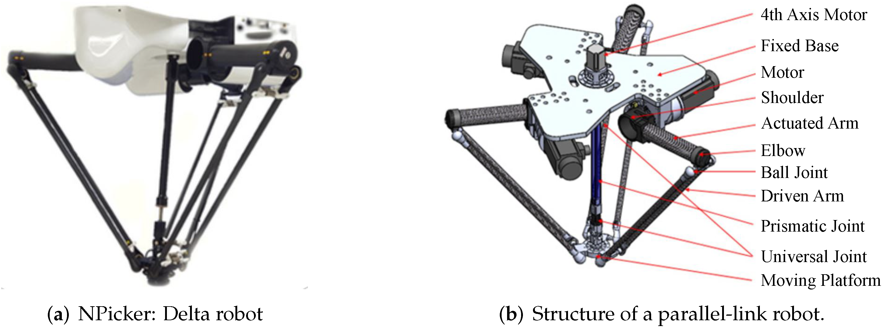
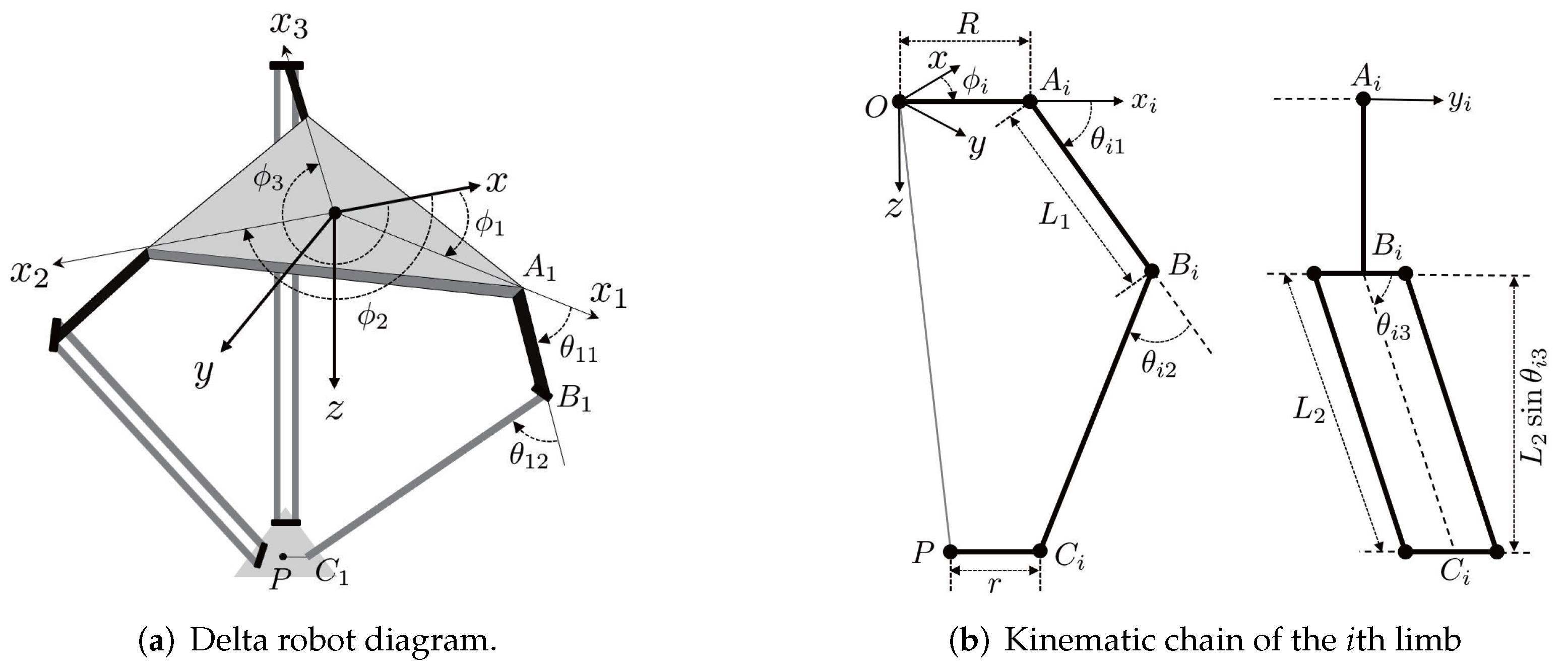
The parallel-link manipulator shown in Figure 1 is a three-degree-of-freedom robot that usually comprises three closed-loop kinematic chains, a fixed base, and a moving platform. Owing to the small mass of the manipulator and three actuators on the fixed base, this parallel-link robot can achieve high precision and high movement speed for pick-and-place tasks. Figure 2b shows the kinematic chain of this robot.
A global reference coordinate system O- is located at the center of the fixed base, where the x- and y axis lie on the fixed base and the z axis points vertically upward. Another coordinate system - () is attached to the fixed base at a distance R (i.e., fixed base radius) along O-, such that the axis is in line with the extension of , the axis is directed along the revolute joint of the elbow, and the axis is parallel to the z axis of O-. Angle for is measured from the x axis to the axis, as depicted in Figure 2a, and is a constant parameter of the robot design measured to be , , and . Let denote the position vector of the centroid P of the moving platform relative to the O- coordinate system. The three joint angles , , and associated with the ith limb are defined as follows: (1) defines the angle of the actuated arm and is measured from the axis to , and (2) and represent the rotating angles of the driven arm . The lengths of the actuated and driven arms are denoted as and , respectively. Let the radii of the fixed base and moving platform be denoted as R and r, respectively. The masses of the actuated arm, driven arm, and moving platform are denoted as , , and , respectively.
The equations of motion of the considered delta robot can be derived using different methods such as Lagrangian equations, virtual work principle, and Newton–Euler methods. Let the vector of the actuator torques to be applied to the active joints at the shoulders in Figure 1b be denoted as . Then, from the Euler–Lagrange formulation based on the energy considerations of robotic systems, the dynamic analytic model can be derived and expressed as follows [9,10,11]: for ,
where Lagrangian multipliers are given as follows:
where denotes sin, and denotes cos in the above expressions. Table 1 lists other parameter values provided by the manufacturer.
Once the path planning of the center of the moving platform determines , , and , the command signal (), that is, the amount of torque that the motor should exert on each parallel link to achieve the trajectory-tracking performance, can be determined as follows:
- From the inverse kinematics analysis given in Appendix B, three active joint angles , , and are numerically obtained.
- By using and and their time derivatives , , , and , Lagrangian multipliers for can be obtained from (2).
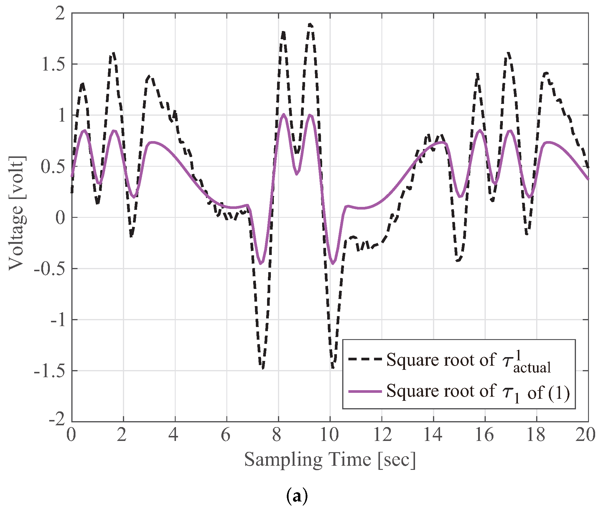
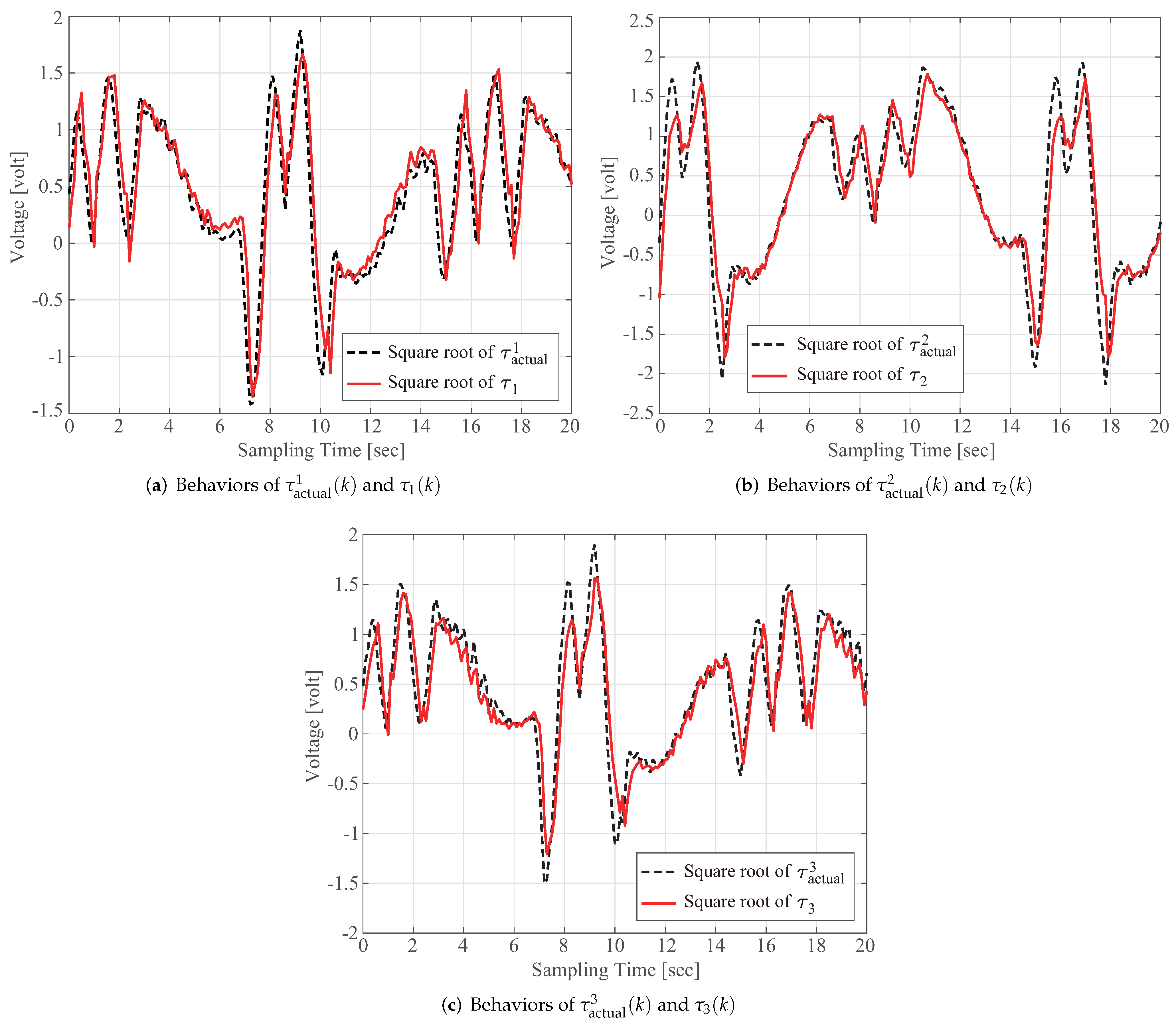
Command signals () that are numerically calculated using (1) by the aforementioned procedure should perfectly match the corresponding actual torque for guaranteeing that the centroid P of the moving platform perfectly tracks the three-dimensional trajectory . In other words, an imprecise value can never provide high tracking performance for the predesigned trajectory of P. Therefore, a thorough similarity evaluation between and is an essential prerequisite for the practical application of delta robots. In this respect, the accuracy of obtained using (1) with the parameter values provided by the manufacturer, as listed in Table 1, is evaluated as follows. The actual torque that is delivered by the implemented motor to the actuated arm cannot be directly determined. Thus, the well-known fact that the torque is proportional to the square of the operating voltage (i.e., ) was introduced in the following experiments. First, the user-selected () was supplied to each motor to activate the parallel-link robot. The dashed line in Figure 3a indicates such a value that is approximately equal to the square root of . Second, the active joint angle was directly measured by sensors during robot operation. Angular velocity and acceleration were calculated from the joint angle data by using central finite difference methods. Lastly, the computed command signal in (1) was obtained by using the parameter values listed in Table 1 and the , , and values. The solid line in Figure 3a denotes the computed voltage that is equivalent to the square root of the computed torque . The discrepancy between and in Figure 3a implies that the amount of torque exerted by the motor with a computed voltage input cannot achieve the high-precision tracking of the predetermined reference trajectory . By contrast, the reference-tracking errors may become small upon the implementation of a suitably designed controller. For example, inverse dynamic control or computed torque control is one of the most effective, well-accepted, and widely used control schemes for rigid robotic manipulator systems to drive the manipulator along the given trajectory as precisely as possible [12]. The key idea of such a control scheme is to introduce feedback linearization to cancel the nonlinear robot dynamics under the assumption that all parameters of the system model are exactly known. Therefore, the inexactness of the model parameters, which can be verified from the discrepancy between and in Figure 3a, results in the degradation of robot performance, even when a model-based motion controller is implemented. Accordingly, the development and identification of a dynamic analytic model of the delta robot are indispensable for calculating actuator torques with high precision. In addition, such an exact dynamic model can contribute to reducing the control effort of model-based controllers required for the trajectory-tracking behavior of robot manipulators.
3. Construction of an Identification-Based Dynamic Model of the Delta Robot
The analytic model structure of the delta robot shown in Figure 1 and Figure 2b was derived using the virtual work principle as follows. Vector for the gravitational force of the moving platform is given as follows:
where g denotes the gravitational acceleration. denotes the equivalent mass of the moving platform and is defined as , where and are the masses of the moving platform and the driven arm, respectively. Vector for the inertia force of the moving platform is obtained as follows:
Further, vector for the gravity torque of the actuated arm is given as follows:
where denotes the length of the actuated arm. denotes the equivalent mass of the actuated arm and is defined as , where is the mass of the actuated arm. Vector for the inertia torque of the actuated arm is
where denotes the inertia matrix of the actuated arm with respect to the fixed frame and is approximately given as follows:
where is an identity matrix of order 3. Let the vector of the virtual angular displacements of joints , , and be denoted by . The vector of the virtual linear displacement of the moving platform is denoted by . Then, the following dynamic model can be derived by applying the virtual work principle [13]:
where . Next, is defined in terms of as follows. The relationship between the velocity of the centroid of the moving platform, , and the actuated joint velocity, , can be written as follows:
where denotes the Jacobian matrix, which is derived as follows. Consider the following constraint condition that can be confirmed easily from Figure 2b [14]: for , 2, and 3,
where denotes the length of the driven arm. Let be the vector written as
where R and r are the radii of the fixed base and moving platform, respectively. Then, (10) can be rewritten as
Therefore, (9) can be derived from (15) as follows:
, defined as (11), depends not only on and , but also on the three-dimensional coordinate of the terminal moving platform. Such a positional coordinate can be obtained by measuring the actuated joint angles (), as described in Appendix A. The derivative of and with respect to time t can be represented as the ratio of an infinitesimal change in time-varying variables. From this fact, it follows that (16) can be expressed as
Because (18) holds for any virtual displacement ,
By contrast, the dynamic model in (19) does not cover all the forces acting on the parallel-link robot; that is, (19) includes only some forces that can be readily analyzed from the rigid-body mechanics [15]. The important forces that are not considered in the aforementioned derivation are those due to friction. Therefore, the aforementioned dynamic model should be extended to at least roughly include the frictional forces in order to render such a model reflect the reality of the physical behavior of the robot and thereby improve the model quality. First, the mathematical model of viscous friction in which each torque in caused by frictional force is proportional to the corresponding actuated joint velocity in , is given as follows:
where () are viscous friction coefficients. Second, the Coulomb friction model is represented as
where () are Coulomb friction coefficients, and denotes a signum function. This model shows that each torque in due to Coulomb friction is constant except for the sign, which depends on the actuated joint velocity. Therefore, the extended formula for joint torques that considers the forces due to friction can be derived from (19), (20), and (21) as follows:
Then, from (3)–(6), (20), (21), and (23), (22) can be rewritten as follows:
where . In conclusion, (25) results in the following form of the joint space dynamic model:
where
where is the inertia matrix, is the matrix of viscous friction coefficients and Coriolis forces, and is the vector of gravity forces and Coulomb friction forces.
The PSO algorithm was inspired by the social and biological behaviors of bird flocks searching for food sources. In this nature-based algorithm, individuals are referred to as particles and fly through the search space seeking the best global position that minimizes (or maximizes) a given problem. The classical PSO algorithm is summarized in Appendix C. Next, the direct estimation of parameters in the derived dynamic model (26) with (27)–(29) using the PSO algorithm in combination with a distributed cyclic neighborhood search, which is a new variant of the aforementioned classical PSO algorithm, is described. Let the vector of the uncertain model parameters to be identified be defined as
Let represent the position vector of each particle in the swarm at the iteration step , where denotes the maximum number of iterations and denotes the particle index. The vector of the sampled measurement of the supplied torques, , is denoted by , where . Further, the sampled measurements of , , and are denoted by , , and , respectively. Then, the estimation of is denoted by . The identification process for developing the dynamic model of a delta robot involves the following steps.
- Step 0.
- Initialize the iteration number as . The position vectors of particles are initialized with randomly chosen . Then, and are, respectively, set as follows:where the predefined even-valued is the number of neighbors of the ith particle, for or . Further, is the objective function that is defined as follows:where the th torque estimation denoted by is calculated from (26)–(29) using the identified parameters in and the discrete measurement data of , , and . The aim of the objective function in (33) is to minimize the deviation between the measurement of the supplied torques and their estimation by employing the joint space dynamic model in (26) with (27)–(29) at each sampling time.
- Step 1.
- Once the termination criterion, set as the total number of iterations performed, is satisfied, the identification process is terminated with the optimal parameters given byOtherwise, the optimization process continues until the termination criterion is satisfied.
- Step 2.
- Each particle in the swarm evolves according to the following equation:where , , and are the inertial factor, cognitive-scaling factor, and social-scaling factor, respectively; and are uniformly distributed random numbers generated separately in the unit interval at each iteration step ℓ; and the initial equals . Then, is updated as follows:Lastly, and are, respectively, updated as follows:Next, go to Step 1 with .
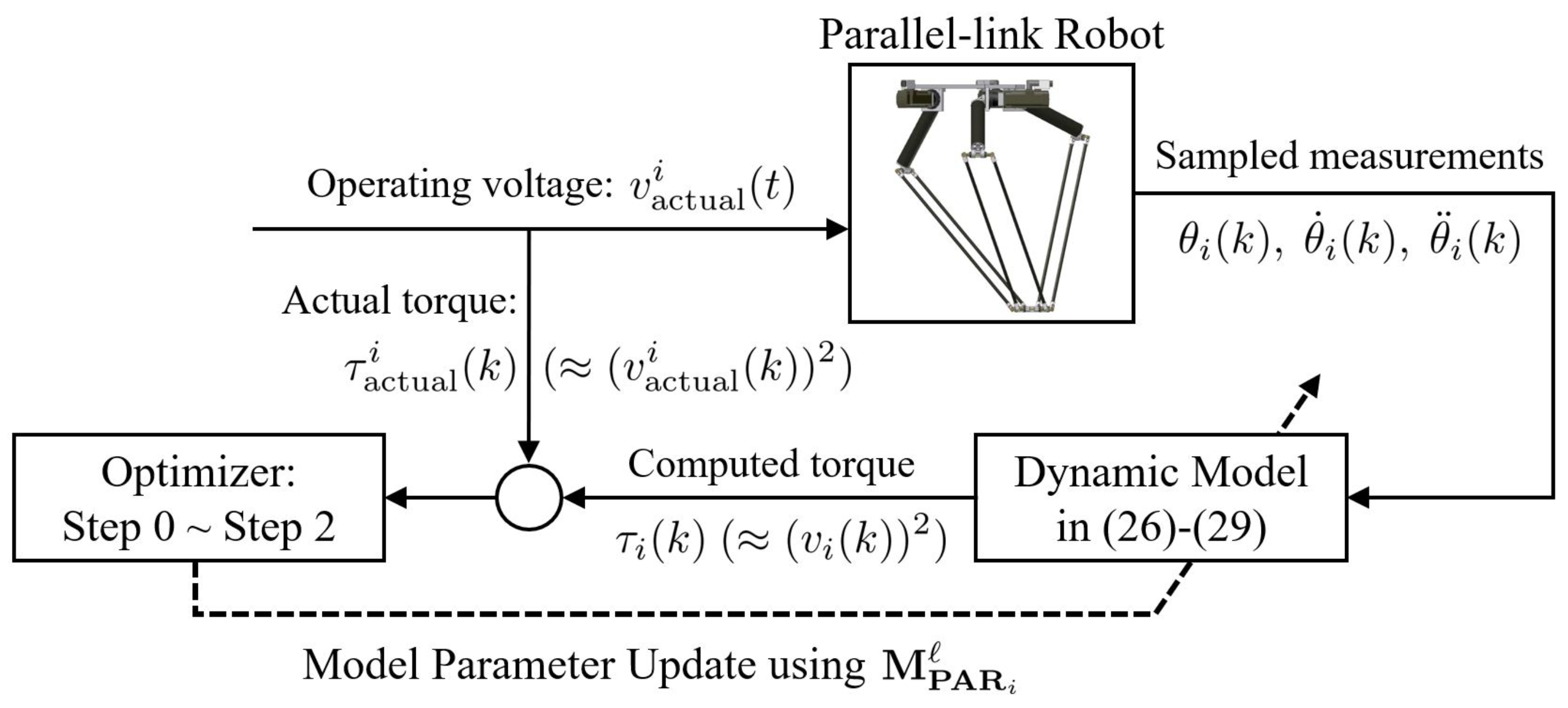
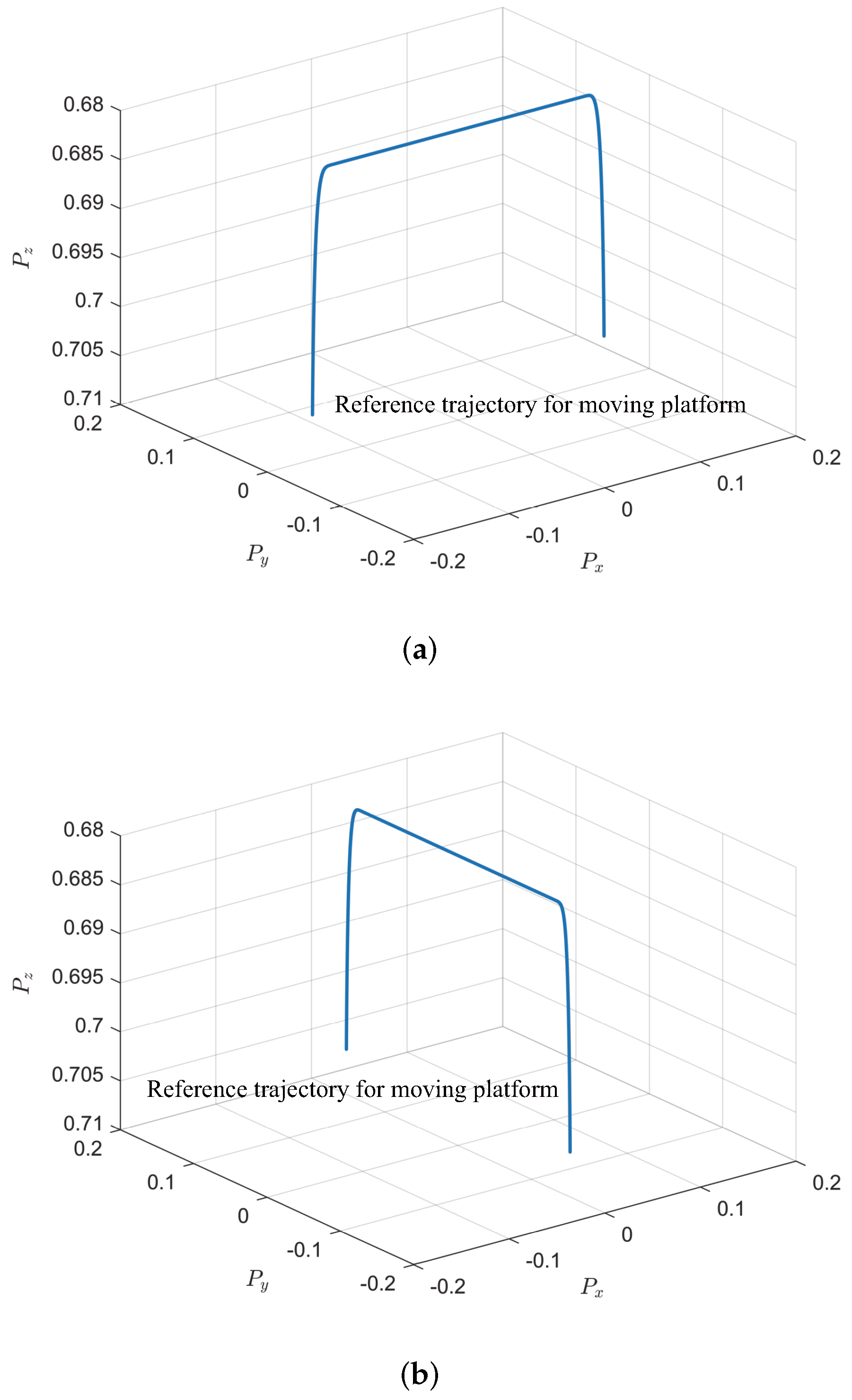
The task is now to determine the optimal parameter vector of in (30) that renders the torque computed from (26) with as close as possible to the applied actual torque obtained from measurements from (, , ) to (, , ). Such a parameter estimation is performed by using the aforementioned PSO-based optimization algorithm and the dataset of [, , ] used for the comparison illustrated in Figure 3a. Figure 4 shows a schematic overview of the experimental setup designed at NT Robot, Co., to measure the actual torque and [, , ] and update the dynamic model parameters via the proposed identification procedure. These data are acquired when the moving platform follows the trajectory shown in Figure 5a. The optimization task for parameter estimation is performed with , , , , and the maximum iteration number of PSO . Then, the identified parameters of the dynamic model (26) with (27)–(29) are obtained as follows:
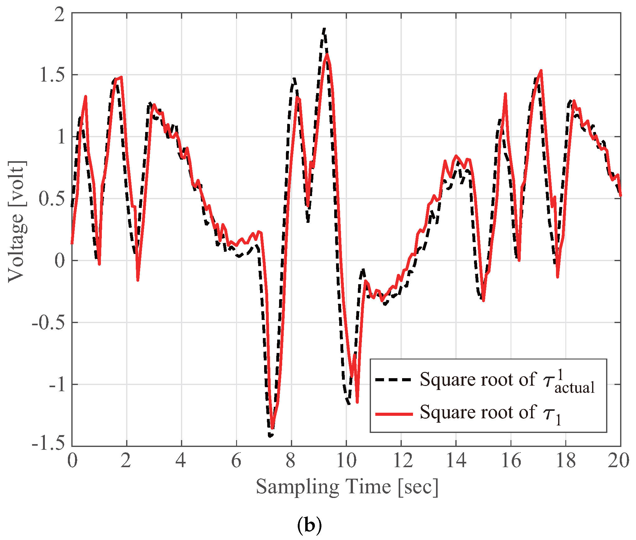
The solid line in Figure 3b shows the characteristics of the computed torque determined from (26) with the estimated parameters in (36). A comparison with the measured actual torque indicates the good fidelity of the derived dynamic model providing . This high model fidelity is attributed to the PSO-based identification scheme introduced for nonlinear dynamic modeling (26) that includes the forces due to viscous and Coulomb frictions.
In summary, our study presented a simple and efficient approach that can directly achieve high-quality identification of an analytic dynamic model for a parallel-link robot. The phrase “simple and efficient” can be characterized from two aspects. First, PSO itself has the advantages of fast search speed, memory, limited parameters, and simple structure. In addition, it is easier to implement at the validation stage than other optimization algorithms are. In addition, the use of PSO facilitates generalized cost functions, which enables the direct identification of a large number of model parameters involved in the analytic dynamic model of delta robots. Second, our identification procedure does not require cumbersome and time-consuming tasks, such as model transformation or development of simulated manipulators used in conventional studies, which can be mainly attributed to the aforementioned flexibility of the PSO algorithm. Thus, our approach is simple and efficient and can directly identify the model parameters effectively. By contrast, the phrase, “high-quality identification”, can be explained as follows. Most robot-related studies that are not based on identification approaches use the physical data provided by manufacturers as model parameters. These physical parameter values often lead to a large discrepancy between the calculated and measured signals, as depicted in Figure 3a. However, with the application of our proposed approach for estimating model parameters, the model can be obtained with high accuracy. This result is experimentally demonstrated in Figure 6, wherein the discrepancy between the calculated and measured signals is considerably smaller than that in Figure 3a. This experimentally demonstrates that our approach enables the achievement of high-quality identification performance.
Remark 1.
The performance degradation of the classical PSO algorithm may mainly be due to the poor particle diversification characteristics, which, in practical implementation, often leads to the potential problem of premature convergence of the swarm to local optima. Diversification enables the optimizer to efficiently explore different regions, possibly resulting in a global search for a good optimum. However, most population-based evolutionary computation techniques, including PSO, depend on the principle of reducing the search space in the progression toward the global optima. Because of the swarm-movement pattern, after a certain number of evolutionary iterations, offspring that outperform their parents can no longer be produced; thus, all the particles remain trapped in a region that may not even contain the local optima. In such cases, if population diversity is not enhanced, particles evolving according to the conventional PSO mechanism may find reaching the true global optimal position challenging. On the basis of this background, the distributed cyclic neighborhood-search mechanism serves as a diversity-boosting tool in our PSO algorithm. This mechanism enables a particle to share information through a “nearby-neighbor” interaction with a series of successively numbered particles, with the particle as the center. In this structure, a particle’s nearby neighbors are not necessarily particles that are close to each other in the hyperdimensional search space. Instead, nearby neighbors are particles that share information on individual fitness values. Thus, the key improvement in the particles’ exploration abilities (or population diversity) in our PSO method can be attributed to their local social learning from their respective neighborhoods, rather than their learning from only one global best particle in the swarm, as in the canonical star topology.
Remark 2.
Although the total number of particles, , is selected through an empirical approach, a systematic method may be required for our PSO algorithm to be more successful. Recently, Kononova et al. [16] revealed and quantified structural bias that, if present, would predispose the algorithm toward limiting its search to specific regions of the solution space. Their result would be useful in determining the suitable swarm size in this PSO scheme. However, the system-identification problem for a delta robot is solved via a one-run optimization process, which implies that the dynamic model is obtained through off-line system identification. Therefore, compared to online identification requiring computational efficiency, the computational complexity may not be a critical issue in this approach. Accordingly, the maximal number of iterations was set as a termination criterion in our study.
4. Discussion
To demonstrate the superiority of the proposed identification scheme, the conventional identification of a parallel robot proposed by Angel and Viola [5] is introduced. Their techniques for the parametric identification of the analytical dynamic model were mainly based on the RLS algorithm. With the aforementioned aim, the nonlinear dynamic model for a delta robot is formulated in the form of the linear regression model. From (1), we have
where
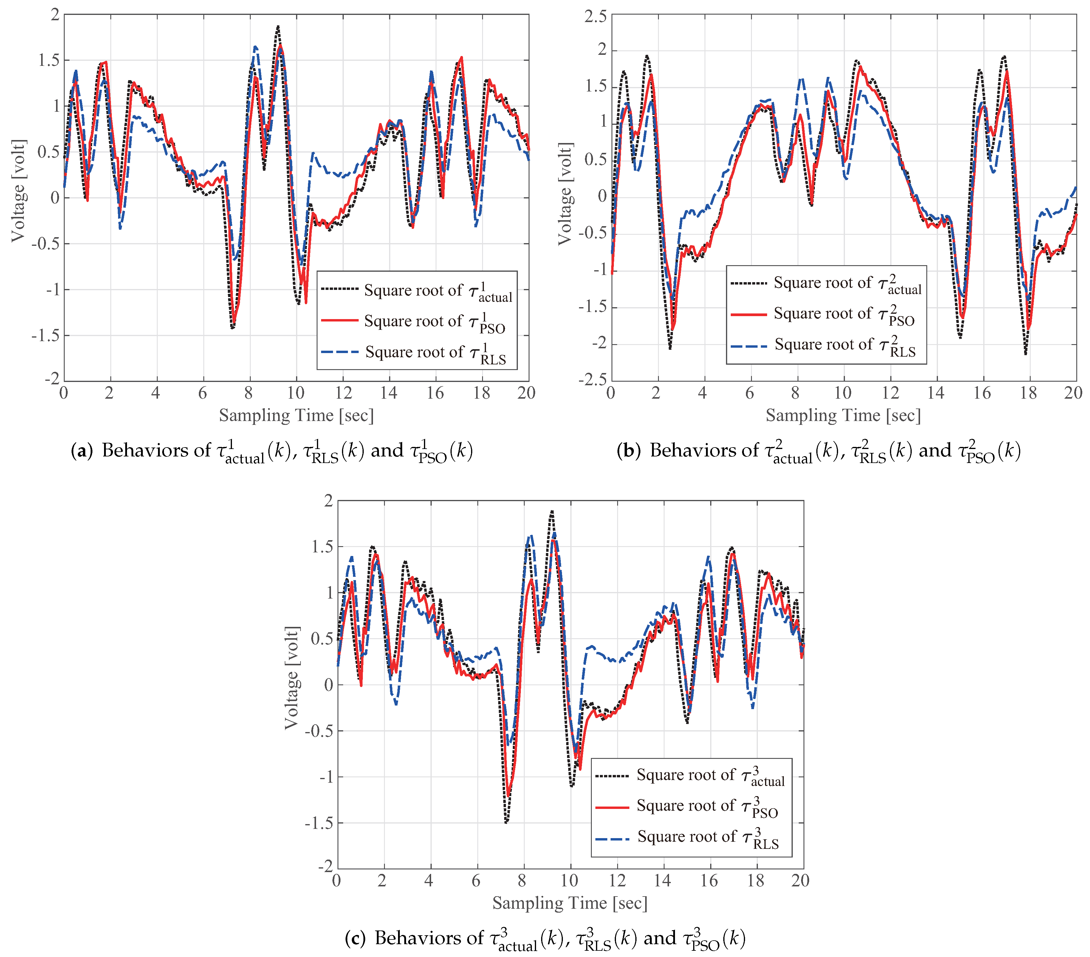
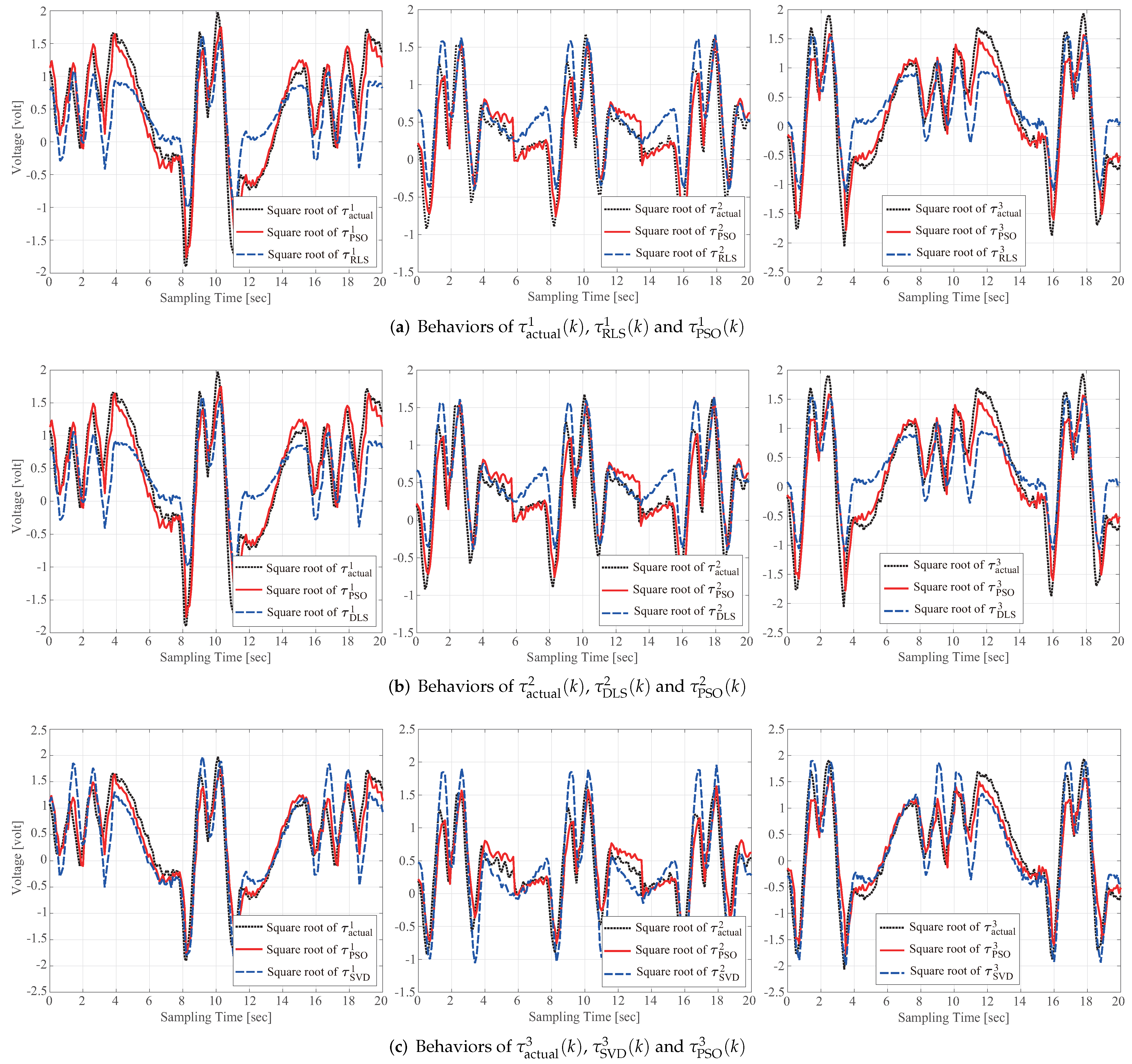
For the above linear regression model, the RLS algorithm presented in Islam and Bernstein [17] is applied, which yields the computed torque () shown in Figure 7, where denotes the torque computed using our identification results. These experimental results clearly demonstrate that our identification scheme outperforms the conventional RLS-based method.
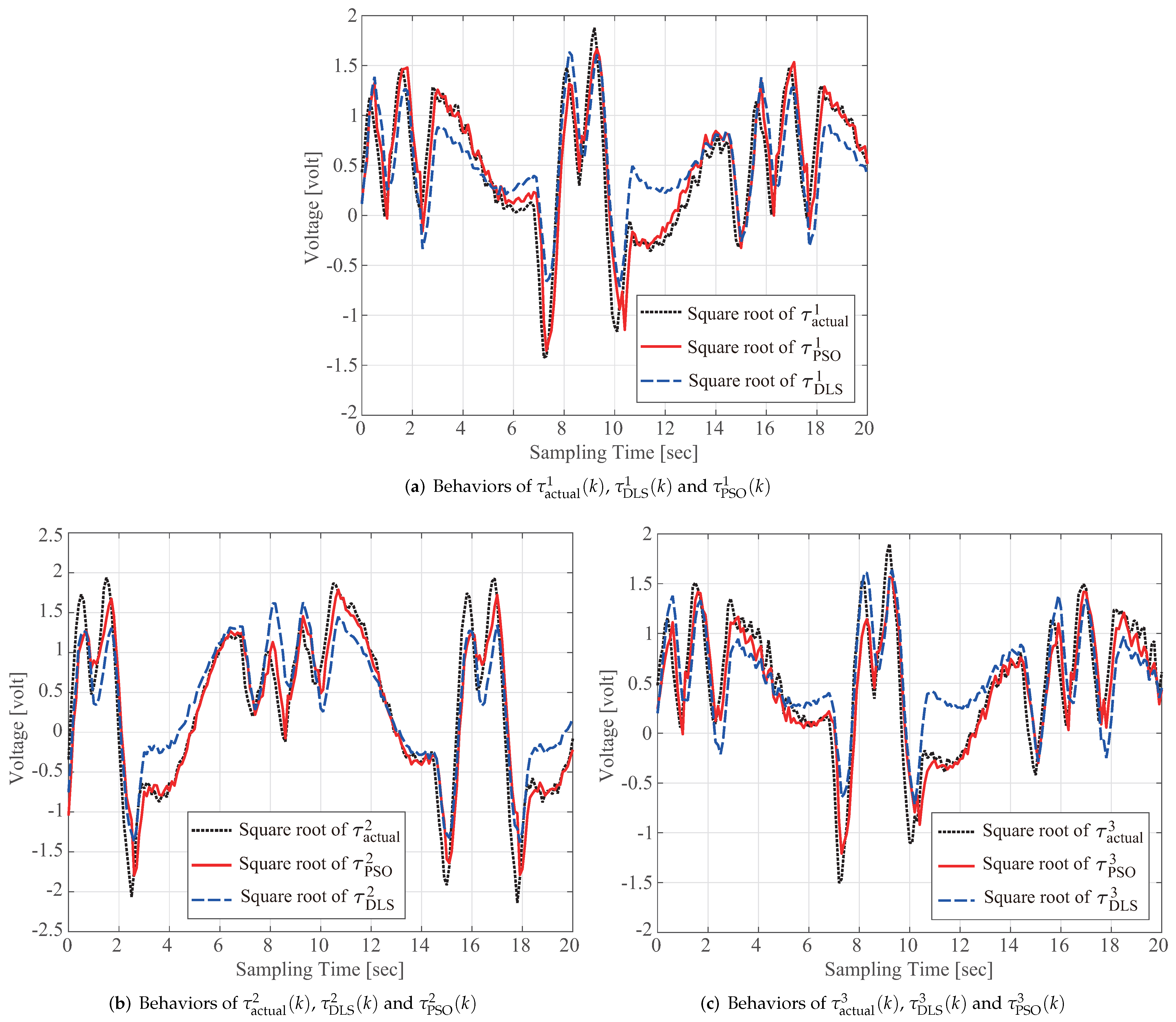
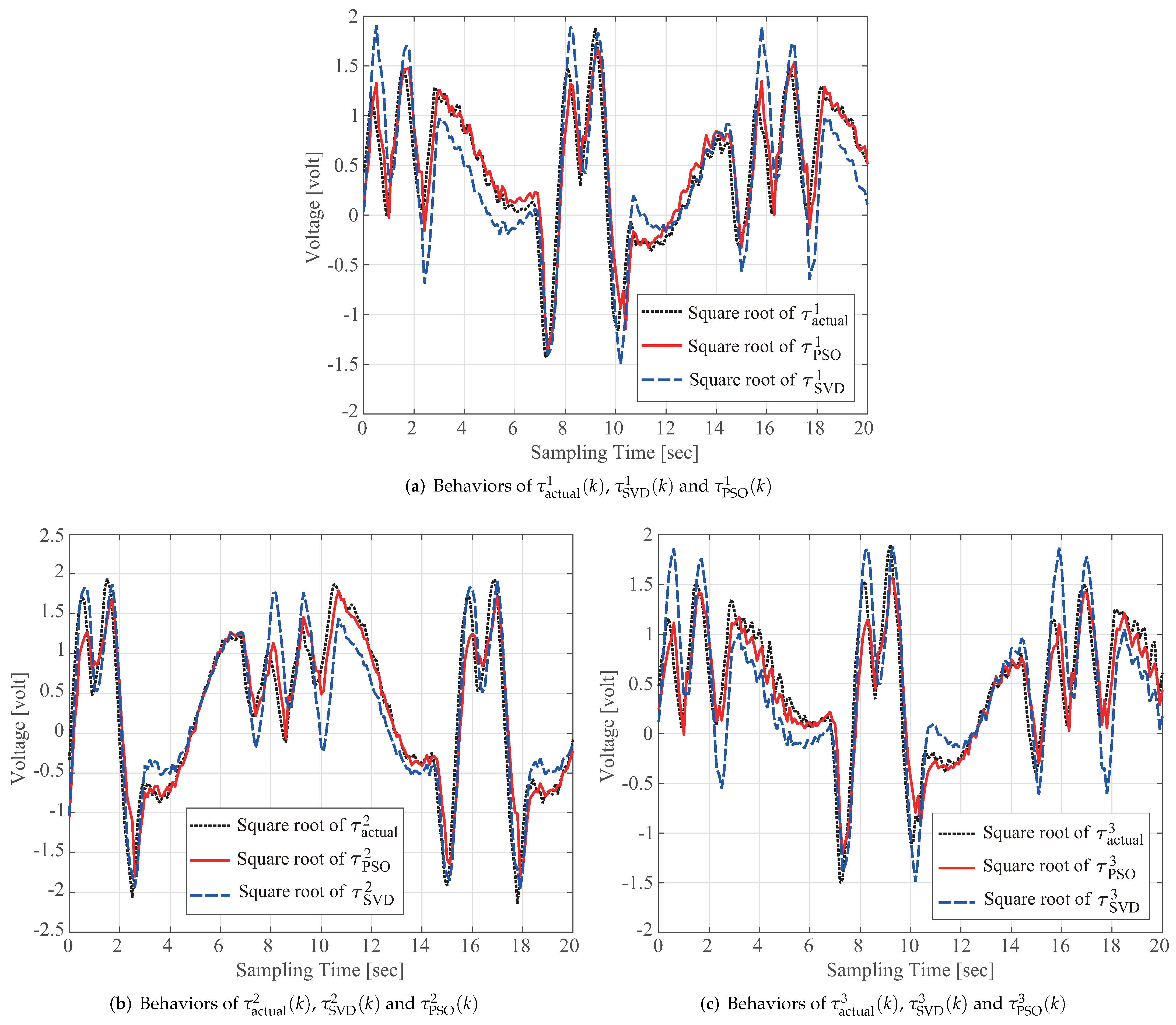
To further validate the high-quality identification performance of the proposed scheme, two other identification methods are examined. The first is the damped least-squares (DLS) method-based identification [18], and the second is the SVD method for least-squares identification [19]. Figure 8 and Figure 9 present the computed torques and , respectively, for . The above examinations clearly verify that the proposed identification scheme for a delta robot achieved better performance compared with the identification results obtained via conventional DLS- and SVD-based identification methods.
Lastly, to further illustrate the superiority of the presented identification scheme, the model validation is performed by using the actual torque and [, , ], which are measured when the moving platform follows the reference trajectory given in Figure 5b. Figure 10 summarizes the model validation results of the PSO-, RLS-, DLS-, and SVD-based identification methods, which demonstrates the validity of our PSO-based identification scheme. The normalized root mean square error (NRMSE) index is introduced to quantitatively evaluate the model fitness, and results were calculated on the basis of the following equation for and are listed in Table 2:
where the notation “*” denotes PSO, RLS, DLS, or SVD, and and are the maximal and minimal elements of the sampled data from the computed torque . A value for (41) close to 1 indicates less variance between the actual torque and model-based computed torque; thus, Table 2 verifies that the proposed scheme outperforms the conventional identification method.
5. Conclusions
In this study, an efficient and reliable parameter-identification method was proposed for the analytic dynamic model of a delta robot. The complex dynamic equations of motion were derived according to the virtual work principle and then extended to characterize the inertial and centripetal/Coriolis forces and the frictional effects on the robot’s dynamic behavior. To directly identify the set of uncertain parameters included in such a dynamic model, the PSO algorithm with a distributed cyclic neighborhood-search mechanism was employed. Compared to conventional methods, our identification technique exhibits the following distinctive features: (i) Owing to the flexibility of the PSO algorithm, the task of transforming the system of equations into a linear formulation with respect to the uncertain system parameters is not necessary. (ii) No cumbersome and time-consuming tasks, such as developing an additional robot-simulation model solely for identifying the parameters in an overdetermined set of equations, are required. The experimental results indicate that the proposed technique can directly achieve high-quality identification of an analytic dynamic model for a parallel-link robot.
Author Contributions
Conceptualization and methodology, T.-H.K. and M.K.; software and experiments, T.-H.K., Y.K. and T.K.; validation and formal analysis, M.K., Y.K. and T.K.; writing—original draft preparation, T.-H.K. and M.K.; writing—review and editing, T.-H.K.; funding acquisition, T.-H.K. All authors have read and agreed to the published version of the manuscript.
Funding
This research was supported by National Research Foundation of Korea (NRF) grant funded by the Korea government (MSIT) (no. 2021R1A2C1008686) and the Chung-Ang University Graduate Research Scholarship in 2021.
Conflicts of Interest
The authors declare no conflict of interest.
Appendix A. Forward Kinematics of the Delta Robot
In this section, the forward kinematics of the delta robot is derived. The vector loop-closure equation of the kinematic chain for the ith limb is expressed as follows:
Rewriting the vector components of (A1) in the coordinate system - gives
Three equations in (A2) are squared and summed to eliminate the passive joint angle as follows:
where
Then, subtracting Equation (A3) of the first kinematic chain (i.e., ) from those of the second () and third () kinematic chains gives
respectively, where , , , and for . Then, Equations (A5) and (A6) can be written in matrix form as follows:
Therefore, and can be obtained in terms of as follows:
Appendix B. Inverse Kinematics of the Delta Robot
In this section, the derivation of the inverse kinematics of a delta robot is presented. Consider Equation (A2). From the second row of (A2), angle is calculated as
By contrast, rewriting (A2) gives
Then, three equations in (A10) are squared and summed to obtain
Appendix C. Classical Particle Swarm Optimization Algorithm
The classical PSO algorithm is a population-based stochastic computational technique with a powerful global-search capability for resolving the following form of the optimization problem without constraints:
where the linear or nonlinear objective function is minimized with respect to the vector of the design variables . Therefore, a particle in the PSO algorithm represents a potential solution in (A13). Let denote the limited subregion of an entire n-dimensional Euclidean space and be assumed to contain the optimal solutions. The conventional evolutionary PSO searching mechanism is initiated with a swarm randomly generated over the space . Thereafter, each particle moves in a coordinated manner through the -dimensional search space. The behavior of each particle is mainly influenced by both its own best previous experience and a social compulsion to move toward a single best particle from the entire swarm as follows:
where denotes the index of the particle; represents the iteration number; and denote the position and velocity vectors, respectively, for the ith particle at the kth iteration; denotes the vector of the best previous position yielding the minimum fitness value for the ith particle; denotes the vector of the global best position determined by the entire swarm; denotes the inertia weight, with and representing the cognitive and social-scaling parameters, respectively; and and are the random parameters generated uniformly in the range of .
References
- Liu, C.; Cao, G.; Qu, Y. Safety analysis via forward kinematics of delta parallel robot using machine learning. Saf. Sci. 2019, 117, 243–249. [Google Scholar] [CrossRef]
- Coronado, E.; Maya, M.; Cardenas, A.; Guarneros, O.; Piovesan, D. Vision-based control of a delta parallel robot via linear camera-space manipulation. J. Intell. Robot. Syst. 2017, 85, 93–106. [Google Scholar] [CrossRef]
- Khalil, W.; Dombre, E. Modeling Identification and Control of Robots; Hermes Penton Ltd.: London, UK, 2002. [Google Scholar]
- Wu, J.; Wang, J.; You, Z. An overview of dynamic parameter identification of robots. Robot. Comput. Integr. Manuf. 2010, 26, 414–419. [Google Scholar] [CrossRef]
- Angel, L.; Viola, J. Parametric identification of a delta type parallel robot. In Proceedings of the 2016 IEEE Colombian Conference on Robotics and Automation (CCRA), Bogota, Colombia, 29–30 September 2016; pp. 1–6. [Google Scholar]
- Liu, Y.; Wu, J.; Wang, L.; Wang, J. Parameter identification algorithm of kinematic calibration in parallel manipulators. Adv. Mech. Eng. 2016, 8, 1687814016667908. [Google Scholar] [CrossRef] [Green Version]
- Mata, V.; Farhat, N.; Díaz-Rodríguez, M.; Manipilators, P. Dynamic parameter identification for parallel manipulators. In Parallel Manipulators, Towards New Applications; IntechOpen: London, UK, 2009; pp. 21–43. [Google Scholar]
- Kim, T.-H.; Byun, J.-I. Truss sizing optimization with a diversity-enhanced cyclic neighborhood network topology particle swarm optimizer. Mathematics 2020, 8, 1087. [Google Scholar] [CrossRef]
- Kuo, Y.-L. Mathematical modeling and analysis of the Delta robot with flexible links. Comput. Math. Appl. 2016, 71, 1973–1989. [Google Scholar] [CrossRef]
- Angel, L.; Viola, J. Fractional order PID for tracking control of a parallel robotic manipulator type delta. ISA Trans. 2018, 79, 172–188. [Google Scholar] [CrossRef] [PubMed]
- Park, S.B.; Kim, H.S.; Song, C.; Kim, K. Dynamics modeling of a Delta-type parallel robot (ISR 2013). In Proceedings of the ISR 2013—44th International Symposium on Robotics, Seoul, Korea, 24–26 October 2013; pp. 1–5. [Google Scholar]
- Ruderman, M.; Iwasaki, M.; Song, C.; Chen, W. Motion-control techniques of today and tomorrow: A review and discussion of the challenges of controlled motion. IEEE Ind. Electron. Mag. 2020, 14, 41–55. [Google Scholar] [CrossRef]
- Li, Y.; Xu, Q. Dynamic analysis of a modified DELTA parallel robot for cardiopulmonary resuscitation. In Proceedings of the 2005 IEEE/RSJ International Conference on Intelligent Robots and Systems, Edmonton, AB, Canada, 2–6 August 2005; pp. 233–238. [Google Scholar]
- Codourey, A. Dynamic modelling and mass matrix evaluation of the DELTA parallel robot for axes decoupling control. In Proceedings of the IEEE/RSJ International Conference on Intelligent Robots and Systems, IROS ’96, Osaka, Japan, 4–8 November 1996; pp. 1211–1218. [Google Scholar]
- Craig, J. Introduction to Robotics: Mechanics and Control, 3rd ed.; Pearson Prentice Hall: Hoboken, NJ, USA, 2005. [Google Scholar]
- Kononova, A.V.; Corne, D.W.; De Wilde, P.; Shneer, V.; Caraffini, F. Structural bias in population-based algorithms. Inf. Sci. 2015, 298, 468–490. [Google Scholar] [CrossRef] [Green Version]
- Islam, S.A.U.; Bernstein, D.S. Recursive least squares for real-time implementation [Lecture Notes]. IEEE Control Syst. Mag. 2019, 39, 82–85. [Google Scholar] [CrossRef]
- Argha, A.; Ye, L.; Cao, K.; Su, S.W.; Celler, B.G. Real-time identification of heart rate responses via auxiliary-model-based damped RLS scheme. In Proceedings of the 2017 39th Annual International Conference of the IEEE Engineering in Medicine and Biology Society (EMBC), Jeju Island, Korea, 11–15 July 2017; pp. 1312–1315. [Google Scholar]
- Yaacoub, F.; Abche, A.; Karam, E.; Hamam, Y. MRI reconstruction using SVD in the least square sense. In Proceedings of the 2008 21st IEEE International Symposium on Computer-Based Medical Systems, Jyvaskyla, Finland, 17–19 June 2008; pp. 47–49. [Google Scholar]
Figure 1.
High-speed pick-and-place parallel-link robot designed at NT Robot, Co.

Figure 2.
Schematics of the Delta robot.

Figure 3.
Measured actual torque is compared with (a) torque (1) calculated using the parameters listed in Table 1 and (b) torque computed using (26) with the estimated parameters in (36). (a) The behavior of computed using (1) with the parameters listed in Table 1. (b) The behavior of computed using (26) with the parameters listed in (36).


Figure 4.
Schematic overview of the system structure for identification of the dynamic analytic model.
Figure 4.
Schematic overview of the system structure for identification of the dynamic analytic model.

Figure 5.
Reference trajectories of moving platform used for identification of the dynamic analytic model and model validation. (a) Reference trajectory for model parameter identification. (b) Reference trajectory for model validation.
Figure 5.
Reference trajectories of moving platform used for identification of the dynamic analytic model and model validation. (a) Reference trajectory for model parameter identification. (b) Reference trajectory for model validation.

Figure 6.
Comparison of the measured actual torque and the torque computed using (26) with the identified parameter values in (36).

Figure 7.
Comparison of the measured actual torque , the torque obtained from RLS-based identification, and the torque computed using (26) with the identified parameter values in (36).

Figure 8.
Comparison of the measured actual torque , the torque obtained from damped least-squares (DLS)-based identification, and the torque computed using (26) with the identified parameter values in (36).

Figure 9.
Comparison of the measured actual torque , the torque obtained from SVD-based identification, and the torque computed using (26) with the identified parameter values in (36).

Figure 10.
Comparison of the actual torque , the torque obtained from RLS-based identification, the torque obtained from DLS-based identification, the torque obtained from SVD-based identification, and the torque computed using (26) with the identified parameter values in (36).


Table 1.
Parameter values provided by the manufacturer for the dynamic analytic model in (1).
Table 1.
Parameter values provided by the manufacturer for the dynamic analytic model in (1).
| Parameter | Value | Unit |
|---|---|---|
| Mass of actuated arm () | kg | |
| Mass of driven arm () | kg | |
| Mass of moving platform () | 2.033 | kg |
| Length of actuated arm () | 0.3423 | m |
| Length of mass center of actuated arm () | m | |
| Radius of moving platform (r) | 0.045 | m |
| Radius of fixed base (R) | 0.2 | m |
| Mass moment of inertia of actuated arm () | kg·m | |
| Motor inertia with gear ratio () | kg·m |
Table 2.
Identified model fitness evaluated for each actuator torque.
| Identification Methods | This Study | RLS-Based Method | DLS-Based Method | SVD-Based Method |
|---|---|---|---|---|
| Model fitness for | 0.9240 | 0.8724 | 0.8714 | 0.8545 |
| Model fitness for | 0.9053 | 0.8679 | 0.8684 | 0.8001 |
| Model fitness for | 0.9228 | 0.8761 | 0.8751 | 0.8604 |
Publisher’s Note: MDPI stays neutral with regard to jurisdictional claims in published maps and institutional affiliations. |
© 2022 by the authors. Licensee MDPI, Basel, Switzerland. This article is an open access article distributed under the terms and conditions of the Creative Commons Attribution (CC BY) license (https://creativecommons.org/licenses/by/4.0/).
Share and Cite
MDPI and ACS Style
Kim, T.-H.; Kim, Y.; Kwak, T.; Kanno, M. Metaheuristic Identification for an Analytic Dynamic Model of a Delta Robot with Experimental Verification. Actuators 2022, 11, 352. https://doi.org/10.3390/act11120352
AMA Style
Kim T-H, Kim Y, Kwak T, Kanno M. Metaheuristic Identification for an Analytic Dynamic Model of a Delta Robot with Experimental Verification. Actuators. 2022; 11(12):352. https://doi.org/10.3390/act11120352
Chicago/Turabian StyleKim, Tae-Hyoung, Yeongjae Kim, Taeheon Kwak, and Masaaki Kanno. 2022. "Metaheuristic Identification for an Analytic Dynamic Model of a Delta Robot with Experimental Verification" Actuators 11, no. 12: 352. https://doi.org/10.3390/act11120352
Note that from the first issue of 2016, this journal uses article numbers instead of page numbers. See further details here.